Download the notebook here! Interactive online version:

The EOQ model and uncertainty propagation

We show how to conduct uncertainty propagation for the EOQ model. We can simply import the core function from temfpy.

import matplotlib.pyplot as plt
import matplotlib as mpl
import seaborn as sns
import chaospy as cp

from temfpy.uncertainty_quantification import eoq_model

Setup

We specify a uniform distribution centered around \(\mathbf{x^0}=(M, C, S) = (1230, 0.0135, 2.15)\) and spread the support 10% above and below the center.

marginals = list()
for center in [1230, 0.0135, 2.15]:
    lower, upper = 0.9 * center, 1.1 * center
    marginals.append(cp.Uniform(lower, upper))

Independent parameters

We now construct a joint distribution for the the independent input parameters and draw a sample of \(1,000\) random samples.

distribution = cp.J(*marginals)
sample = distribution.sample(10000, rule="random")

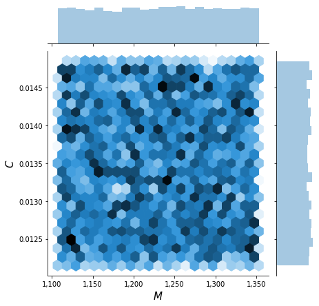
The briefly inspect the joint distribution of \(M\) and \(C\).

plot_joint(sample)

We are now ready to compute the optimal economic order quantity for each draw.

y = eoq_model(sample)

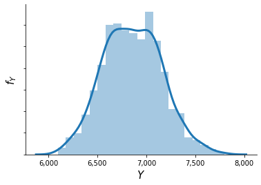
This results in the following distribution \(f_{Y}\).

plot_quantity(y)

Depdendent paramters

We now consider dependent parameters and construct their joint distribution using a Gaussian copula.

corr = [[1.0, 0.6, 0.2], [0.6, 1.0, 0.0], [0.2, 0.0, 1.0]]
copula = cp.Nataf(distribution, corr)

We are ready to sample from the distribution.

sample = copula.sample(1000, rule="random")

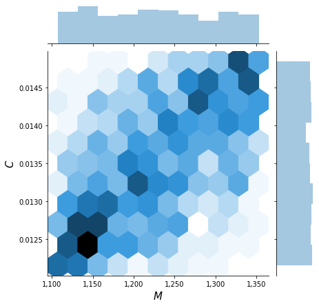
Again, we briefly inspect the joint distribution which now clearly shows a dependence pattern.

plot_joint(sample)

y = eoq_model(sample)

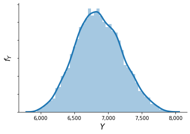
This now results in a distribution of \(f_{Y}\) where the peak is flattened out.

plot_quantity(y)