Download the notebook here!
Interactive online version: ![]()
Quantitative sensitivity analysis
Generalized Sobol Indices
Here we show how to compute generalized Sobol indices on the EOQ model using the algorithm presented in Kucherenko et al. 2012. We import our model function from temfpy and use the Kucherenko indices function from econsa.
[1]:
import matplotlib.pyplot as plt  # noqa: F401
import numpy as np

from temfpy.uncertainty_quantification import eoq_model

# TODO: Reactivate once Tim's PR is ready.
# from econsa.kucherenko import kucherenko_indices  # noqa: E265
The function kucherenko_indices expects the input function to be broadcastable over rows, that is, a row represents the input arguments for one evaluation. For sampling around the mean parameters we specify a diagonal covariance matrix, where the variances depend on the scaling of the mean. Since the variances of the parameters are unknown prior to our analysis we choose values such that the probability of sampling negative values is negligible. We do this since the EOQ model is not
defined for negative parameters and the normal sampling does not naturally account for bounds.
[2]:
def eoq_model_transposed(x):
    """EOQ Model but with variables stored in columns."""
    return eoq_model(x.T)

mean = np.array([1230, 0.0135, 2.15])
cov = np.diag([1, 0.000001, 0.01])

# indices = kucherenko_indices( # noqa: E265
#    func=eoq_model_transposed, # noqa: E265
#    sampling_mean=mean,  # noqa: E265
#    sampling_cov=cov,  # noqa: E265
#    n_draws=1_000_000,  # noqa: E265
#    sampling_scheme="sobol",  # noqa: E265
# )  # noqa: E265
Now we are ready to inspect the results.
[4]:
# fig # noqa: E265
Shapley Effects
Here we show how to compute Shapley effects using the EOQ model as referenced above. We adjust the model in temfpy to accomodate an n-dimensional array for use in the econsa Shapley effects context.
[5]:
# import necessary packages and functions
import numpy as np
import pandas as pd
import chaospy as cp
import matplotlib.pyplot as plt
import seaborn as sns

from econsa.shapley import get_shapley
from econsa.shapley import _r_condmvn
Load all neccesary inputs for the model, you will need: - a vector of mean estimates - a covariance matrix - the model you are conducting SA on - the functions x_all and x_cond for conditional sampling. These functions depend on the distribution from which you are sampling from - for the purposes of this illustration, we will sample from a multivariate normal distribution, but the functions can be tailored to the user’s specific needs.
[6]:
# mean and covaraince matrix inputs
n_inputs = 3
mean = np.array([5.345, 0.0135, 2.15])
cov = np.diag([1, 0.000001, 0.01])
[7]:
# model for which senstivity analysis is being performed
def eoq_model_ndarray(x, r=0.1):
    """EOQ Model that accepts ndarray."""
    m = x[:,0]
    c = x[:,1]
    s = x[:,2]
    return np.sqrt((24 * m * s) / (r * c))
[8]:
# functions for conditional sampling
def x_all(n):
    distribution = cp.MvNormal(mean, cov)
    return distribution.sample(n)

def x_cond(n, subset_j, subsetj_conditional, xjc):
    if subsetj_conditional is None:
        cov_int = np.array(cov)
        cov_int = cov_int.take(subset_j, axis = 1)
        cov_int = cov_int[subset_j]
        distribution = cp.MvNormal(mean[subset_j], cov_int)
        return distribution.sample(n)
    else:
        return _r_condmvn(n, mean = mean, cov = cov, dependent_ind = subset_j, given_ind = subsetj_conditional, x_given = xjc)
[9]:
# estimate Shapley effects using the exact method
method = 'exact'
np.random.seed(1234)
n_perms = None
n_output = 10**4
n_outer = 10**3
n_inner = 10**2

exact_shapley = get_shapley(method, eoq_model_ndarray, x_all, x_cond, n_perms, n_inputs, n_output, n_outer, n_inner)
[10]:
exact_shapley
[10]:
| Shapley effects | std. errors | CI_min | CI_max | |
|---|---|---|---|---|
| X1 | 0.814539 | 0.003178 | 0.808311 | 0.820768 |
| X2 | 0.130068 | 0.003394 | 0.123416 | 0.136721 |
| X3 | 0.055392 | 0.004386 | 0.046797 | 0.063988 |
[11]:
# estimate Shapley effects using the random method
method = 'random'
np.random.seed(1234)
n_perms = 25000
n_output = 10**4
n_outer = 1
n_inner = 3


random_shapley = get_shapley(method, eoq_model_ndarray, x_all, x_cond, n_perms, n_inputs, n_output, n_outer, n_inner)
[12]:
random_shapley
[12]:
| Shapley effects | std. errors | CI_min | CI_max | |
|---|---|---|---|---|
| X1 | 0.814734 | 0.004659 | 0.805602 | 0.823866 |
| X2 | 0.130517 | 0.004570 | 0.121561 | 0.139473 |
| X3 | 0.054749 | 0.004739 | 0.045461 | 0.064038 |
Now we plot the ranking of the Shapley values below.
[14]:
# plot for exact and random permutations methods
ranking(data = df)
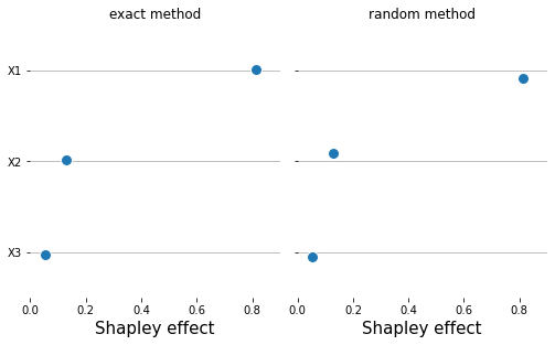
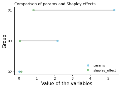
As noticed above, both methods produce the same ranking. Sometimes, it is neccesary to compare the parameter estimates with their parameter values. A typical thing to want to check for is whether the parameter estimates are significant, and what the contribution of significant / insignificant estimates is to the output variance as reflected by their Shapley ranking.
We can plot the parameter estimates together with their Shapley ranking as shown below:
[16]:
# plot exact method comparison
ranking_params_shapley(ordered_df)

[18]:
# plot random method comparison
ranking_params_shapley(ordered_df)
When do I use which method?
The exact method is good for use when the number of parameters is low, depending on the computational time it takes to estimate the model in question. If it is computationally inexpensive to estimate the model for which sensitivity analysis is required, then the exact method is always preferable, otherwise the random is recommended. A good way to proceed if one suspects that the computational time required to estimate the model is high, having a lot of parameters to conduct SA on is
always to commence the exercise with a small number of parameters, e.g. 3, then get a benchmark of the Shapley effects using the exact method. Having done that, repeat the exercise using the random method on the same vector of parameters, calibrating the n_perms argument to make sure that the results produced by the random method are the same as the exact one. Once this is complete, scale up the exercise using the random method, increasing the number of parameters to the
desired parameter vector.
Quantile Based Sensitivity Measures
We show how to compute global sensitivity measures based on quantiles of model’s output.
[19]:
# import necessary packages and functions
import numpy as np
import pandas as pd
import chaospy as cp
import matplotlib.pyplot as plt
import seaborn as sns

from temfpy.uncertainty_quantification import eoq_model
from econsa.quantile_measures import mc_quantile_measures
Firstly, we specify the parameters of the function. This function mc_quantile_measures is capable of computing numerical results of quantile-based sensitivity measures on various user-provided models. Here we take EOQ model from temfpy as an example, where the model function is adjusted to accommodate an n-dimensional array. For multivariate distributed samples, the loc and scale keywords are denoted by a mean vector and a covariance matrix respectively. Considering both
efficient computation and good convergence, we set n_draws equal to 3000 and \(2^{13}\) for brute force and double loop reordering estimators correspondently. Note that the double loop reordering estimator is more efficient than the brute force estimator.
[20]:
# model to perform quantile based sensitivity ananlysis
def eoq_model_transposed(x):
    """EOQ Model but with variables stored in columns."""
    return eoq_model(x.T)
[21]:
# mean and covaraince matrix inputs
mean = np.array([5.345, 0.0135, 2.15])
cov = np.diag([1, 0.000001, 0.01])
n_params = len(mean)
dist_type = "Normal"
Then we are ready to calculate the numerical results using the algorithm presented in Kucherenko et al. 2019.
[22]:
# compute quantile measures using brute force estimator
bf_measures = mc_quantile_measures("brute force", eoq_model_transposed, n_params, mean, cov, dist_type, 3000,)
[23]:
bf_measures
[23]:
| x_1 | x_2 | x_3 | ||
|---|---|---|---|---|
| Measures | alpha | |||
| q_1 | 0.020 | 64.010462 | 10.595192 | 6.522037 |
| 0.052 | 53.565287 | 11.764802 | 7.126140 | |
| 0.084 | 47.203635 | 11.849184 | 7.315335 | |
| 0.116 | 43.584702 | 11.945758 | 7.390247 | |
| 0.148 | 40.746792 | 12.074625 | 7.493912 | |
| ... | ... | ... | ... | ... |
| Q_2 | 0.852 | 0.851180 | 0.108055 | 0.040765 |
| 0.884 | 0.857788 | 0.102897 | 0.039315 | |
| 0.916 | 0.863797 | 0.099314 | 0.036889 | |
| 0.948 | 0.871352 | 0.093822 | 0.034825 | |
| 0.980 | 0.880632 | 0.089250 | 0.030119 |
124 rows × 3 columns
[24]:
# compute quantile measures using double loop reordering estimator
dlr_measures = mc_quantile_measures("DLR", eoq_model_transposed, n_params, mean, cov, dist_type, 2 ** 13,)
[25]:
dlr_measures
[25]:
| x_1 | x_2 | x_3 | ||
|---|---|---|---|---|
| Measures | alpha | |||
| q_1 | 0.020 | 64.179809 | 10.414823 | 6.285291 |
| 0.052 | 52.267399 | 11.037341 | 6.778817 | |
| 0.084 | 46.311146 | 11.211302 | 6.917412 | |
| 0.116 | 42.563103 | 11.407816 | 7.013578 | |
| 0.148 | 40.321098 | 11.638289 | 7.183969 | |
| ... | ... | ... | ... | ... |
| Q_2 | 0.852 | 0.865417 | 0.097312 | 0.037271 |
| 0.884 | 0.871006 | 0.093422 | 0.035572 | |
| 0.916 | 0.876810 | 0.089801 | 0.033388 | |
| 0.948 | 0.883911 | 0.084970 | 0.031119 | |
| 0.980 | 0.890728 | 0.081605 | 0.027667 |
124 rows × 3 columns
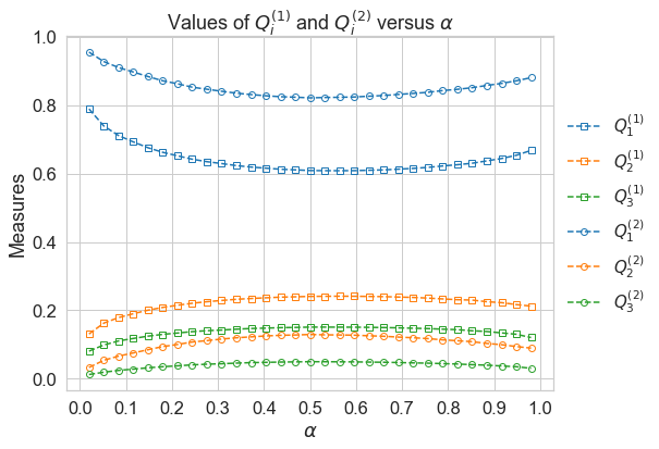
Now we are able to visualize the results.
[27]:
# plot brute force estimates
plot_quantile_measures(bf_measures)
[28]:
# plot double loop reordering estimates
plot_quantile_measures(dlr_measures)
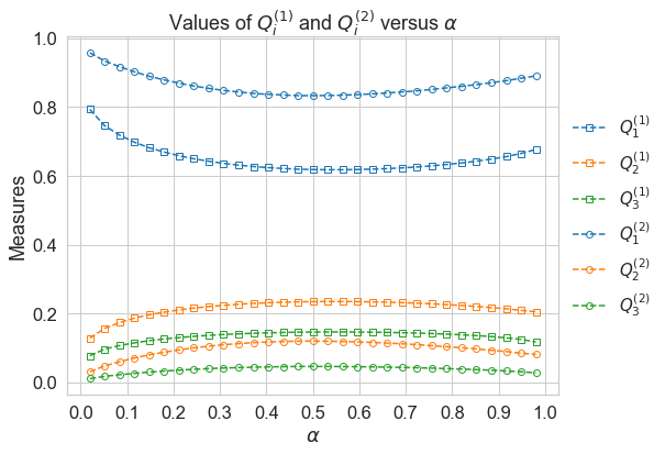
The brute force estimator and DLR estimator generate the same ranking of variables for all quantiles: \(x_1, x_2, x_3\)(in descending order). At \(\alpha=0.5\), measures \(Q_i\) reachs their minimun:\(i=1\) and maximum:\(i=2,3\).